This homework will help a student understand why selling covered calls or cash-secured puts is not income. In fact, the student will see that options are always volatility trades — you will appreciate just how deeply insightful the concept of put-call parity is.
Prerequisites:
basic probability including conditional probability (although you do not need Bayes Thereom, just logic. You will need to do a lot of reasoning the same way you need to turn any word problem into math statements)
Excel or your preferred computational tool
First, a self-indulgent remark…
I enjoy helping people learn about options. Not for instrumental reasons like the “world needs more options traders”. But in an appreciative sense — option theory is a rich toolbox for decision-making in investing and life in general. The word “decision” implies an option.
Notwithstanding, the typical person learning about options is thinking instrumentally — “how do I use these things to make money?” Of course, there’s no blog post or even book-sized answer to this question. As any craft goes, there’s basic vocabulary and principles, but these are necessary but insufficient conditions for success. You need years of trial and error to achieve competence.
Since trading/investing is a low signal-to-noise endeavor your epistemology requires strict discipline — the flip side of narrow bid-ask spreads and low-cost trading means your lack of edge can be masked for a long time. You know a loan shark is a bad deal, so you only visit Sleepy Sal as a last resort. But one broken kneecap and your LTV goes to zero. Brutal but honest. Everyone understands the deal.
Meanwhile, Robinhood administers the morphine of hidden fees to lengthen the duration of its most valuable asset — your overconfidence. Robinhood calls itself Robinhood without a hint of irony. They ate the whole wheel of cheese. I’m not even mad, I’m impressed.
Good news
At risk of pollyanna-posting, I’ll propose just getting smarter. If you have read this far you are totally capable of learning. Unsurprisingly, options discourse either tends to one of 2 poles:
Physics-esque math geekdom
Jargon-heavy complexity certainly has a place in finance but is best ignored as a small ecological niche.
The “option premiums are to be sold for passive income” grift
I’ve covered why this frame is nonsense ad nauseum here, here, here, and indirectly in almost all my writing.
There is a needle to be thread between these framings.
With no more than HS or even middle school math, you have enough tools to tinker and build intuition alongside your live experimentation. This homework is an example of what I’m talking about.
The purpose of this exercise
I get approached for help with options by retail traders frequently. On the one hand, it puts me in an uneasy situation — I’m not really a fan of people using their precious human capital on a machine that conspires to make you think it’s worth trying when base rates say otherwise. On the other hand, who the hell am I to discourage grown-ups who have read the disclaimers and proceed anyway. On balance, it’s a good thing that card-counting books are on the shelves even if most people who fancy themselves Ed Thorp are delusional about what it takes.
So it goes….my sympathies point to being helpful even if the occasional learner impales themselves. They probably would have anyway and there are more people that will be saved by either re-allocating their attention when they realize this is a grind or shed the misunderstandings that keep them plateaued.
All of this really cuts to the heart of Moontower’s approach to unlocking others: part Zen and The Art Of Options Trading, part shedding misunderstandings.
I can’t give you answers, but I can help rule out wrong answers. In that spirit, this exercise, despite its simplicity, will stimulate growth-inducing reflection.
The origin of this exercise
A reader approached me about a strategy they were exploring. It was familiar because it belonged to the class of strategies I’d describe as “harvesting”. Sell some variation of optionality (cash-secured puts, covered calls, iron condors, strangles, etc), earn steady profits.
This reader is selling downside butterflies on the SP500.
When someone has researched a strategy, they are mentally invested in confirming that it works. So right off the bat, I was heartened by the reader’s honest approach — “Kris, tell me what’s wrong with my strategy?”
It’s a fair question. But it’s not quite the right question.
I haven’t done the work so I’m not in the best position to say whether the strategy is good or bad but more importantly…
The “teach a man to fish” Socratic lesson is to demonstrate the implicit misunderstandings of the reader’s approach. That will lead them to higher-resolution questions that will scaffold their ability to answer the original question.
Let’s get to the exercise
Scenario Description
⚙️
Assumptions
A stock is trading for $100.
The risk-free rate and dividends are zero so we can ignore cost of carry or hurdle concerns.
Options on the stock expire after 20 periods. You can think of them as days
How the stock moves
In each period the stock can only go up or down
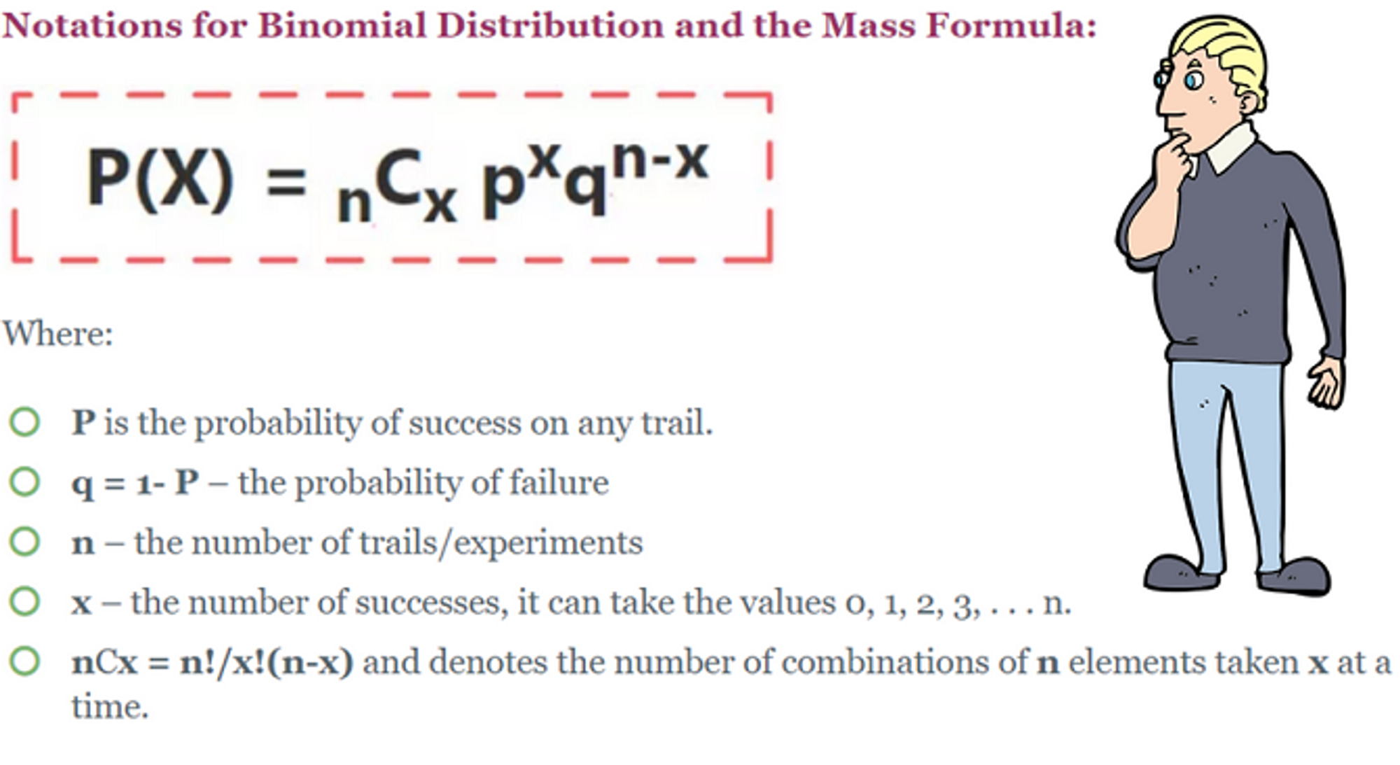
You may want to refresh yourself on coin flips or binomial distribution as encapsulated by this picture:
Probabilities and Magnitude
P(up) = probability stock increases in value = 50%
P(down) = 50%
Magnitude: The stock always moves $1.00
📊
Understanding the distribution
For any single period, the stock is 50% to go up $1 and 50% to go down $1. What’s the expected value of the stock after the first period? After 20 periods? The stock starts at $100
1 period
.50 x $1 + .50 x -$1 = 0 so after the first period the expected value of the stock remains $100.
20 periods
= $100 + 20 * expected profit per trial
= $100 + 20 * $.0
= $100.00
After 20 periods, how many possible outcomes are there?
Hint
My favorite technique — do a simpler version of the problem first.
What’s the sample space after 1 period:
$101 or $99…2 possible outcomes
What’s the sample space after 2 periods:
3 possible outcomes:
Down 2x: $98
Up 2x: $102
Up, down or down, up: $100
Note there are 4 possible paths and 3 possible outcomes. after 2 periods
What’s the sample space after 3 periods:
4 possible outcomes:
$97
Down 3x
$103
Up 3x
$99
Up, down, down
Down, down, up
Down, up, down:
$101
Up, up, down
Down, up, up
Up, down, up
Note there are 8 possible paths and 4 possible outcomes. after 3 periods
Are you seeing a pattern?
Answer to the number of outcomes
Based on the hint you can see the pattern.
For n periods, there are n + 1 outcomes.
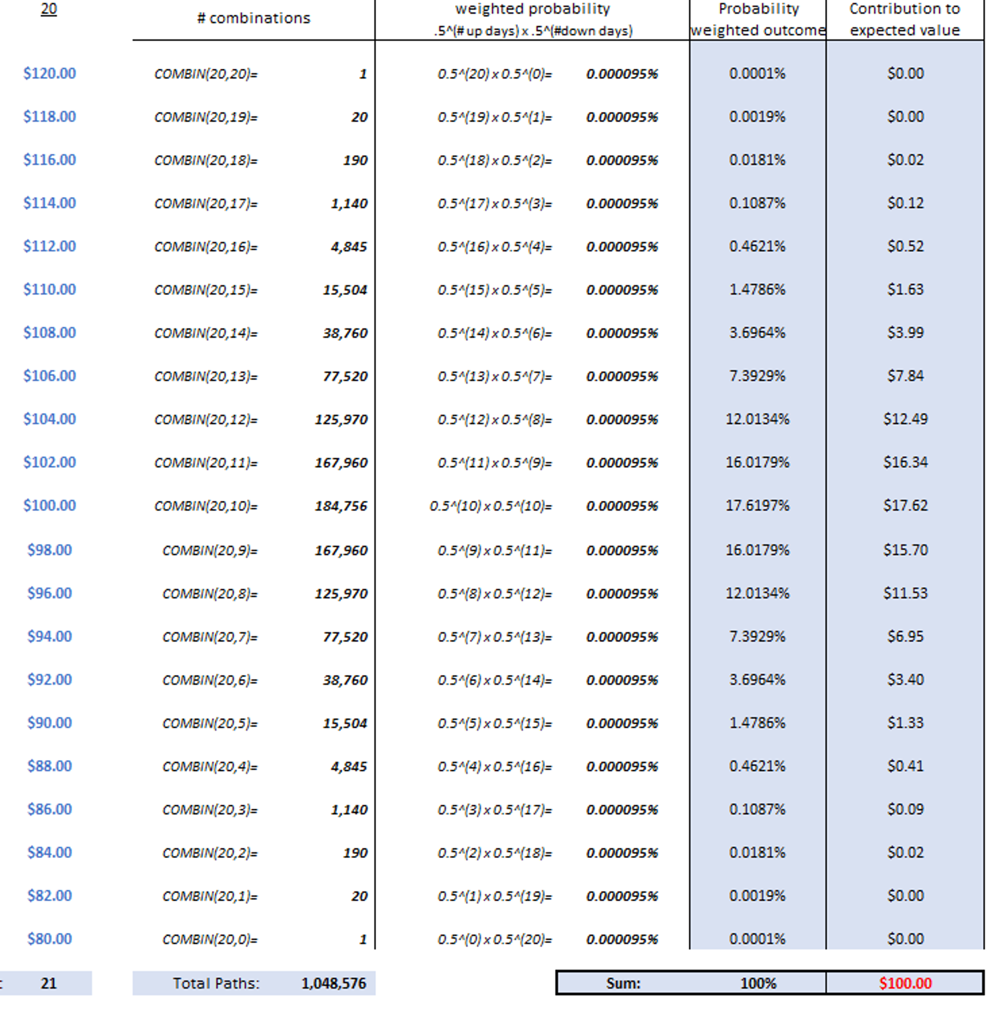
So for 20 periods, there are 21 possible price outcomes.
Answer to the number of paths
Based on the hint you can see the pattern.
For n periods, there are 2ⁿ paths:
1 period = 2 paths
2 periods = 4 paths
3 periods = 8 paths
So for 20 periods, there are 2²⁰ or1,048,576 possible price paths.
Visual answer
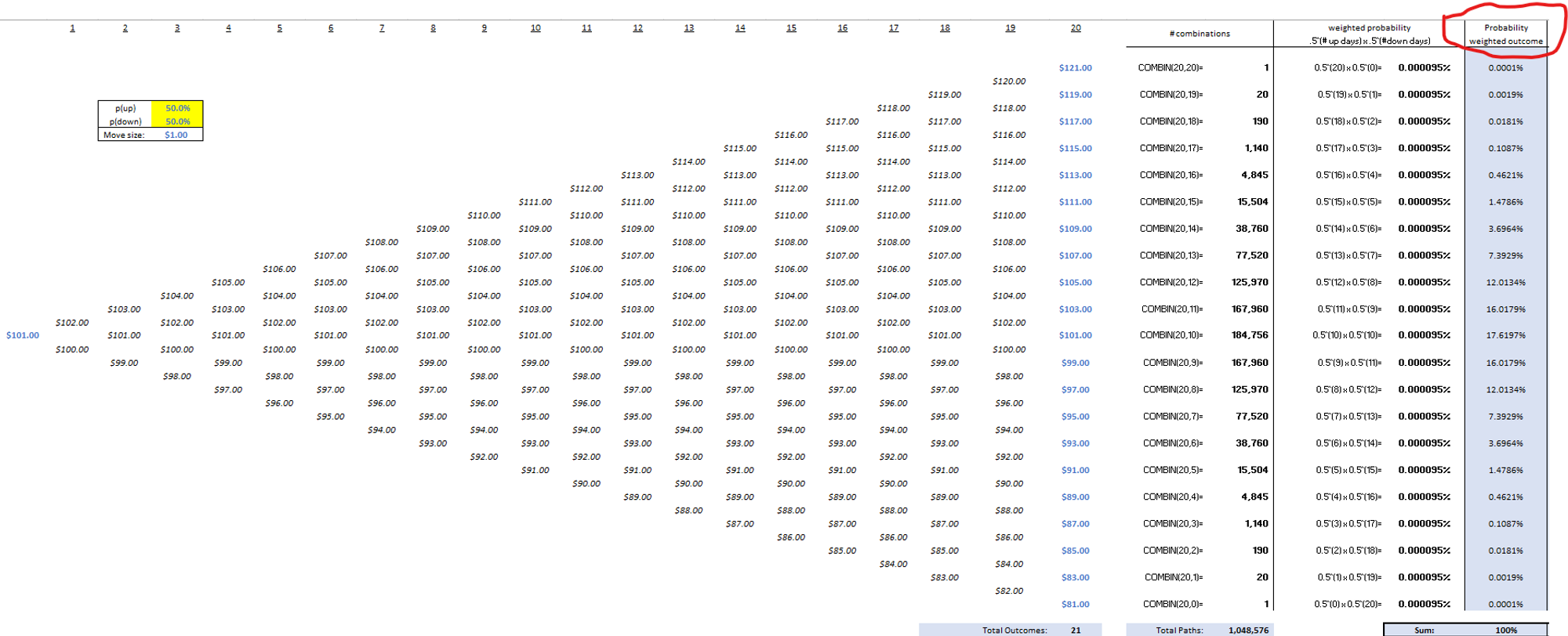
Just like coin flips, this simple up/down model conforms to the basic binomial distribution.
Again, this picture:
While we used 2²⁰ to find the total number of price paths, there are only 21 possible outcomes.
The binomial distibution is represented by a binomial tree. the ₙCₓ term is a coefficient that denotes how many combinations can generate a particular outcome.
A simple example is there is only combin(20,20) or “20 choose 20” ways to have 20 up moves in a row. In other words, only 1 path out of 1,048,576. This is true and symmetrical for 0 heads in a row for 20 straight trials.
A neat trick is you can use Pascal’s Triangle for n = 20 to see all the coefficients instead of computing them with a combination function.
What is the probability of each outcome? This is the distribution.
Hint
The answer again lies in this picture where the up and down probabilities weight the combinations.
Set p = 50% and q = 50%
Answer to the distribution
🧮
The probability-weighted outcome =
(# of combinations) *probability of X up moves * probability of N-X down moves at each outcome
The probability-weighted outcomes sum to 100%.
Remember that, the expected value of the stock after 20 periods is $100.00
You can see how the probability of each outcome times the price at that outcome contributes to an expectancy of $100.
🏒
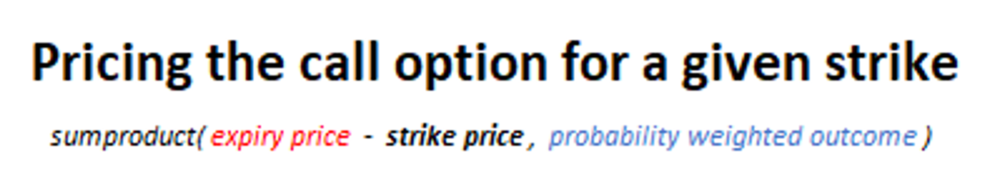
Pricing Options
In this discrete distribution, we know there are 21 possible terminal prices for the stock after 20 periods. By knowing all the possible expiration prices and their probabilities we can price an option for any strike by simply weighting all of the possible payoffs.
🔑
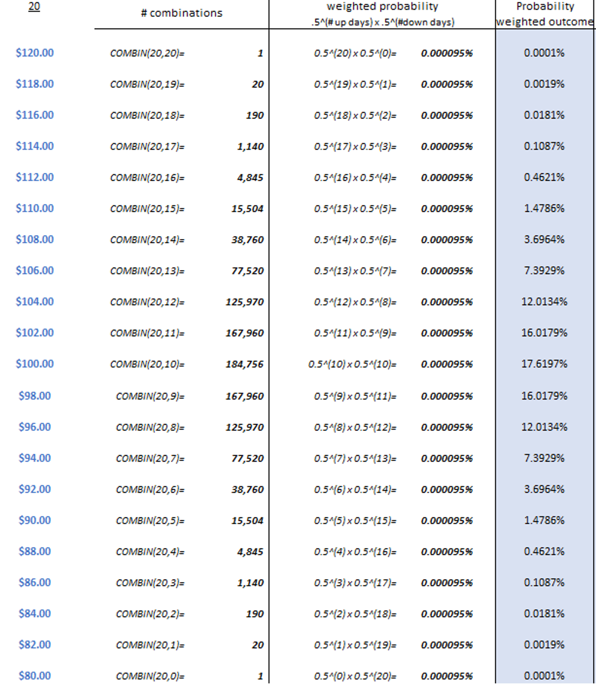
HelpGeneral hint
In case you need to refer to the distribution because you didn’t compute it yourself
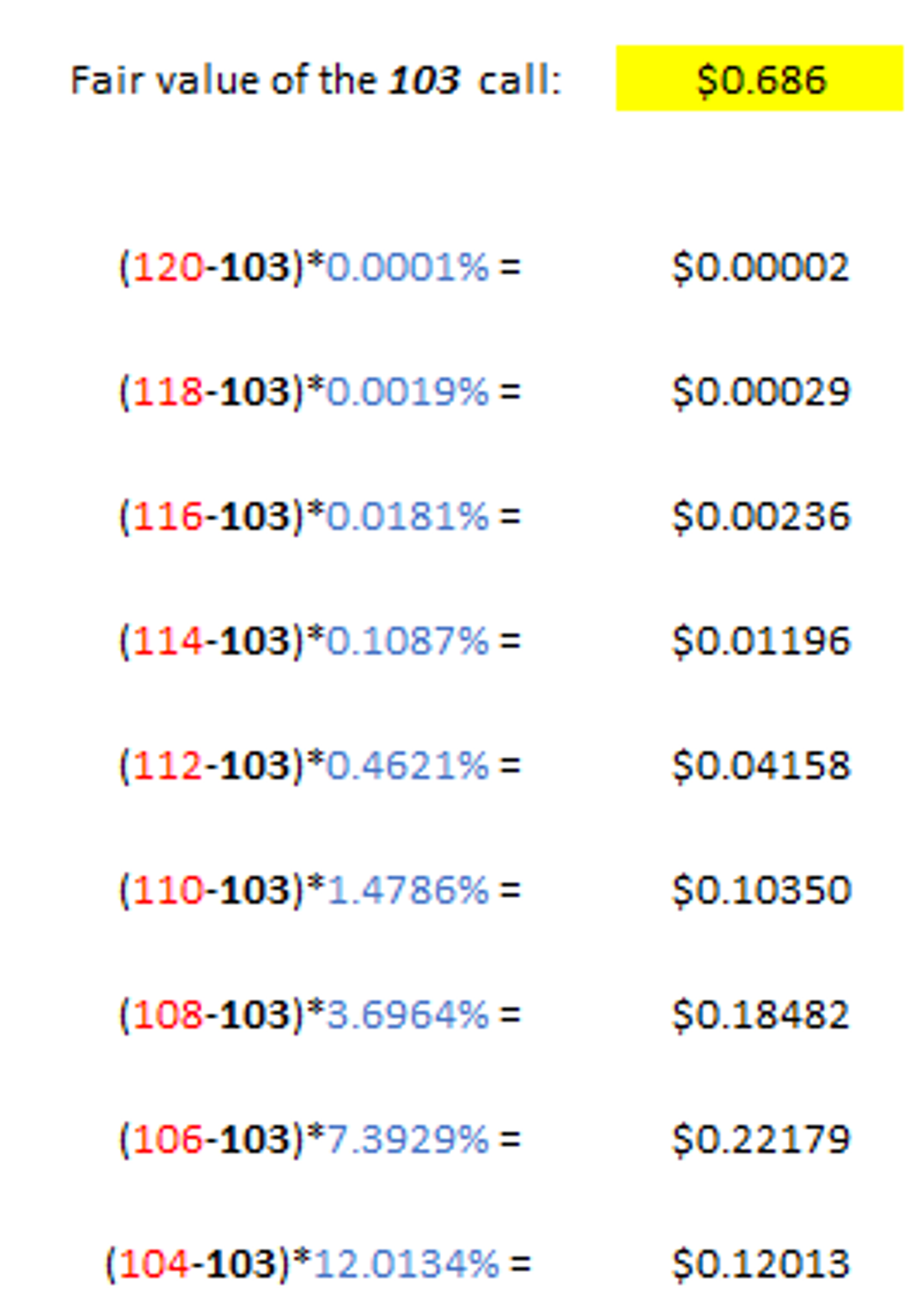
What is the fair value of the 103-strike call at the beginning of the 20 periods when the stock is $100?
Answer
The delta of an option predicts how much the price of the option will change for a $1 change in the stock. In practice, this is an output of an option model such as Black-Scholes and like the formula in general is sensitive to the option’s moneyness, implied volatility, and time to expiry.
But we were able to price the 103-call arithmetically using a binomial tree. We were able to do this because we simplified the stock process into something discrete — either the stock will go up or down $1 each day. We do this because the intuition from such a model is deeply instructive without needing to wade into continuous models and calculus.
Likewise, we can compute delta arithmetically, just as we priced the option.
Here’s your chance.
What’s the delta of the 103 call?
Hint
You originally priced the 103 call with the stock price at $100.
Recall the definition of delta:
Change in option price / $1 change in stock price
Answer
Price of the 103-call with the stock $1 higher (ie $101):
$.938 instead of $.686 when the stock was $100.
Why?
Because the probability of it being in-the-money increased.
Repeat the option valuation calculation you did previously using the updated “probability weighted outcomes” in this table and you will get the $.938 call price.
Note, that for a $1 change in the stock, the option value increased by $.252 corresponding to a 25.2% delta!
Let’s be thorough.
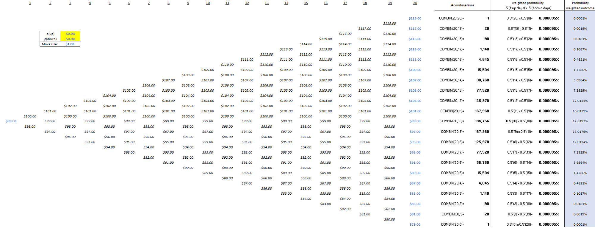
Price of the 103-call with the stock $1 lower (ie $99):
$.435 instead of $.686 when the stock was $100.
Why?
Because the probability of it being in-the-money decreased.
Repeat the option valuation calculation you did previously using the updated “probability weighted outcomes” in this table and you will get the $.435 call price.
Note, that for a $1 change in the stock, the option value decreased by $.251 corresponding to a 25.1% delta!
So the weighted average delta is 25.15%…We will just round the delta to:
25%
So with 20 days until expiry and the stock at $100 the delta of the 103-call is 25%!
[Note if you computed the delta of the call with the same process while assuming the stock price was $101 (and toggled it to $102 to re-compute its value) the delta would be higher than 25%. That’s the effect of gamma — the change in delta itself as the stock price chages!]
💰
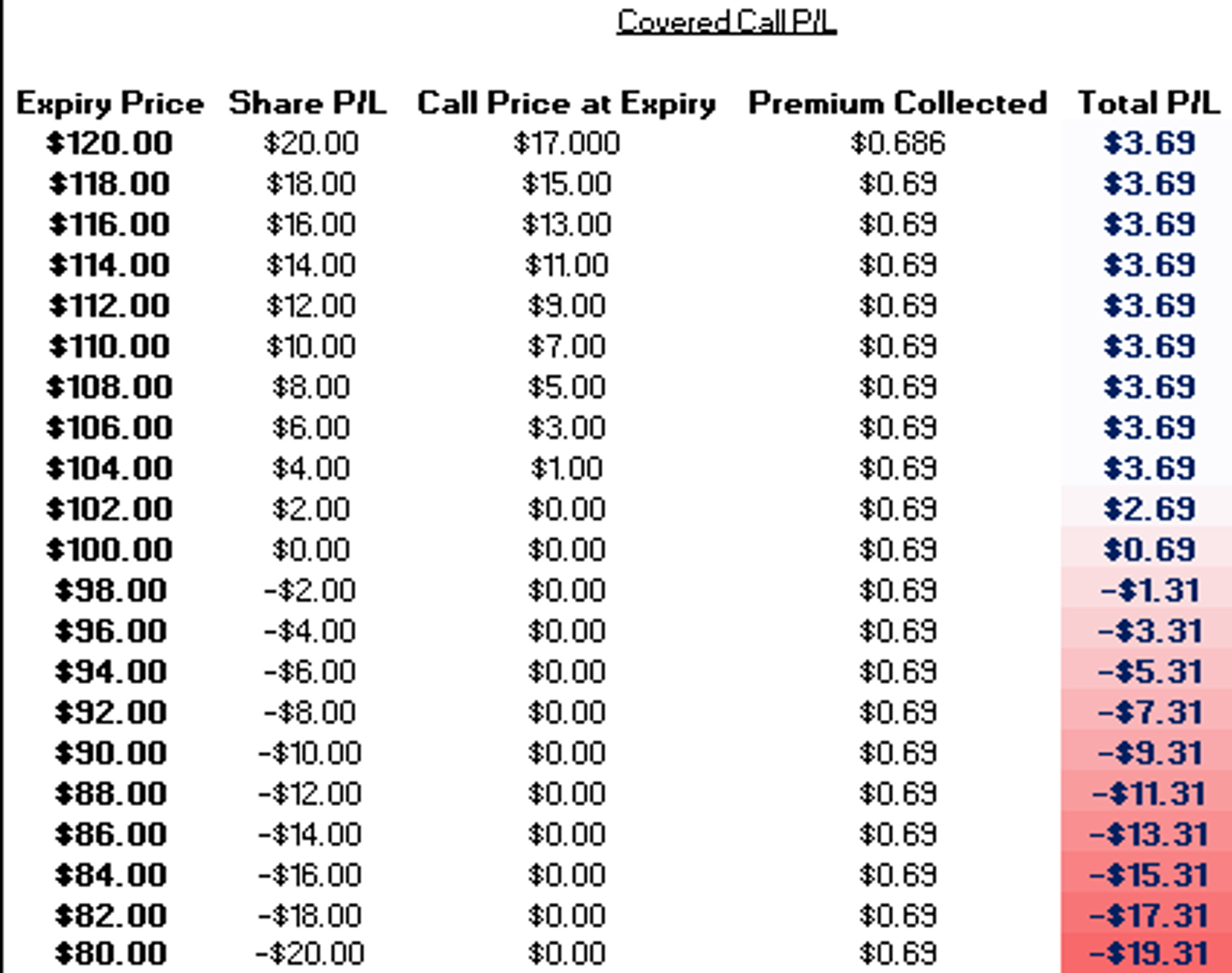
Computing P/Ls
Imagine we sell the 103-strike call as part of a covered call strategy.
Compute the P/L at expiration for each of the 21 terminal prices assuming you own 1 share of the stock (assume you purchased it for $100) and sold the call at its fair value you computed above.
Hints
A call option’s payoff at expiration is the maximum of:
stock price - strike price
zero
or
MAX(S-K, 0)
Answer
Covered Call Strategy P/L =
share P/L - call value at expiry + call premium collected
Recall that the 103 call is worth $.686 (rounding to $.69) from the solution to the prior question.
⏸️
A pause for some words
Assuming you are not a masochist volatility trader, if you sell covered calls you hold a portfolio of long shares, short calls until expiration and maybe you sell calls again for the next term.
What’s going through your brain is “I’m going to own the shares anyway, I might as well receive some premium income, and if I get called away on the shares I’ll be happy anyway.”
To be blunt — this logic is mysterious to me since the whole point of owning equities is for the upside but that’s not really the point of this particular exercise.
Your interest in covered calls is an opportunity to understand how options are intimately about volatility and why you should not use them unless you have a view on volatility that is differentiated from the market’s consensus.
Stay with this exercise and it will all make sense…
We’re doing basic p/l calculations still.
If you own a share of stock and it increases by $1, you enjoy a $1 profit and vice versa.
If you have a covered call strategy, and the stock increases by $1 you make $1 profit on your shares lose on your short calls. If you are short a 25% delta call, it will gain $.25 of value on that same $1 move.
Share position: +$1
Call position: -$.25
Net P/L: +$.75
[If the shares go down in value you will lose $.75 (-$1 on the shares and +$.25 on the short call position.]
The key insight: at the inception of this portfolio you have a 75% exposure to the stock instead of 100%. You make or lose $.75 instead of $1 when the stock moves $1.
If you are a professional options trader explicitly playing the abstract game of “trading volatility” you’d hedge the entire delta…you would not want to have exposure to direction because you have no opinion on the company as an investment.
But the covered call seller clipping some coupon that “averages down their purchase price” or some marketing b.s. like that is now implicitly a volatility trader that just has a long bias.
The difference between this investor and the volatility trader is the investor is not going to continuously rebalance their share position to maintain a constant exposure to the stock.
[the other difference is the investor doesn’t realize they are now a “vol trader” but that’s the point of this whole post — to make this crystal clear]
The volatility trader tries to maintain zero exposure.
The covered call seller who sells a .25 delta call initiates a 75% exposure. However, the exposure is going to bounce around between 0 and 100% depending on how far the stock is from the strike price, how volatile the stock is, and how much time remains.
This is easy to understand at the extremes. If you are short the 103 call and long a share of stock trading for $200 you no longer have any marginal exposure to the price. If the stock goes to $199 or $201 you are unaffected. The owner of the call you are short is the one exposed to the stock. You can think of them as owning the shares that are in your account.
Similarly, if the stock is trading for $10, you own 100% of the exposure. The 103 call you are short is worthless because it’s so far out-of-the-money.
⚖️
Portfolio Comparisons
Because the investor who sells covered calls is not explicitly “trading vol” they are not rebalancing. In our example, they are long the stock, short the .25 delta call, and just close their eyes until expiration.
This provides a perfect Socratic problem to work through to understand why the moment they traded an option they became vol traders.
Let’s continue.
You already computed the p/l for the covered call portfolio for every expiration scenario. The equivalent portfolio exposure that does not use options is to:
Simply sell 25% of your shares and hold the remaining 75%
This portfolio is initially equivalent to the covered call portfolio — it participates at 75% of the stock’s moves. And that will always be true. The covered call portfolio’s net exposure changes, as described earlier, but this is exactly why we can learn what it actually means to trade an option. This comparsion will cut straight to the heart of options.
In sum, there are 2 portfolios:
A) Covered Call Portfolio consisting of:
1 long share from a price of $100
1 short 103-strike call at a price of $.69 (initially a .25 delta call)
B) Reduced Position Portfolio consisting of:
Long .75 of a share
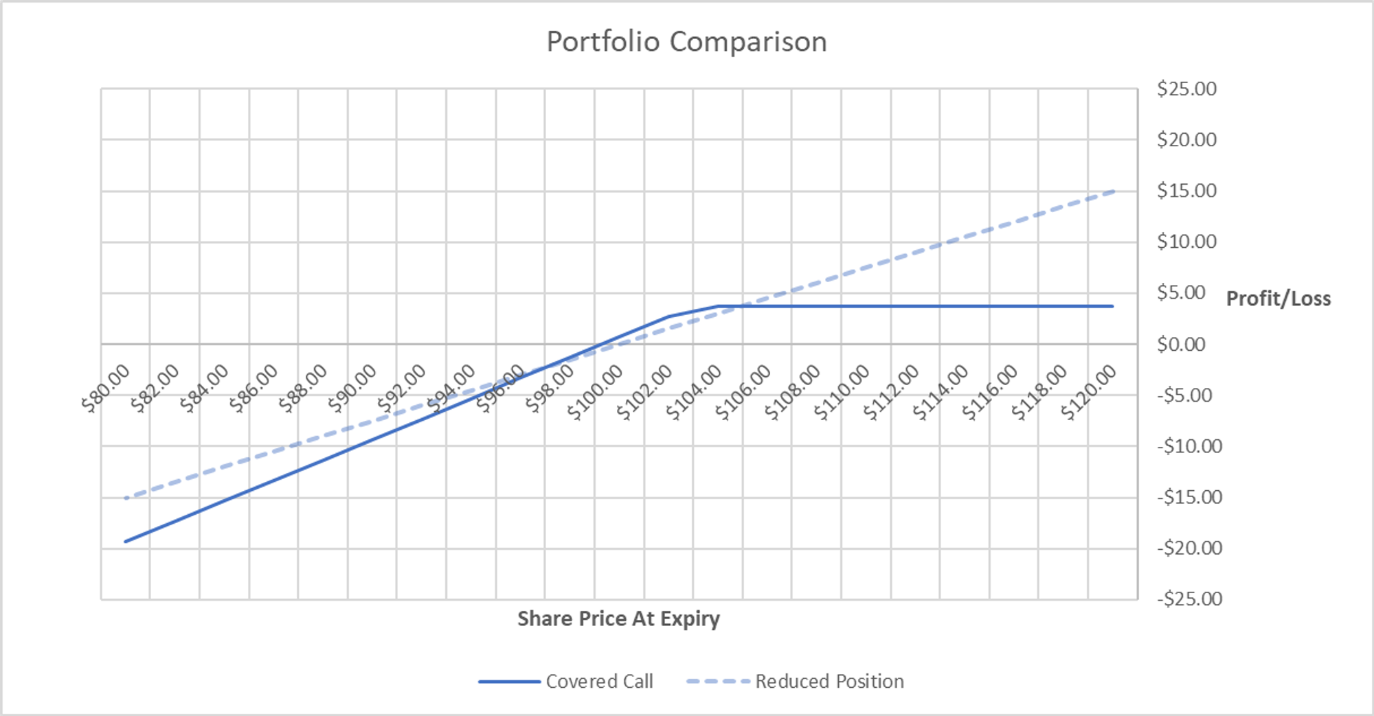
Plot the p/ls of the covered call portfolio vs the portfolio that only maintains a 75% exposure to the stock for every expiration price.
Answer
The Reduced Position portfolio looks as you expect — a typical share exposure except the P/L slope is .75 instead of 1
The Covered Call portfolio has the familiar hockey stick shape we see with options. Specifically it looks like a short put diagram (we’ll talk about put-call parity a touch but a covered call is economically equivalent to a short put). You can see at high share prices the slope of the p/l is zero and at low prices the slope is 1 and in fact steeper than the Reduced Position slope of .75
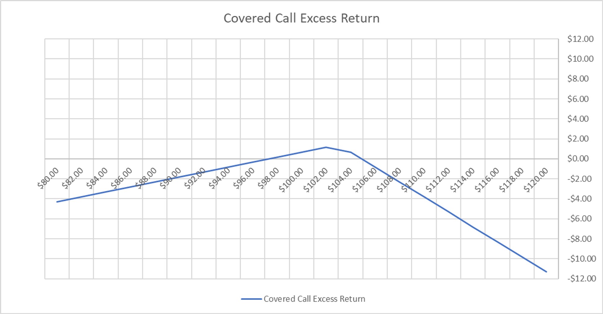
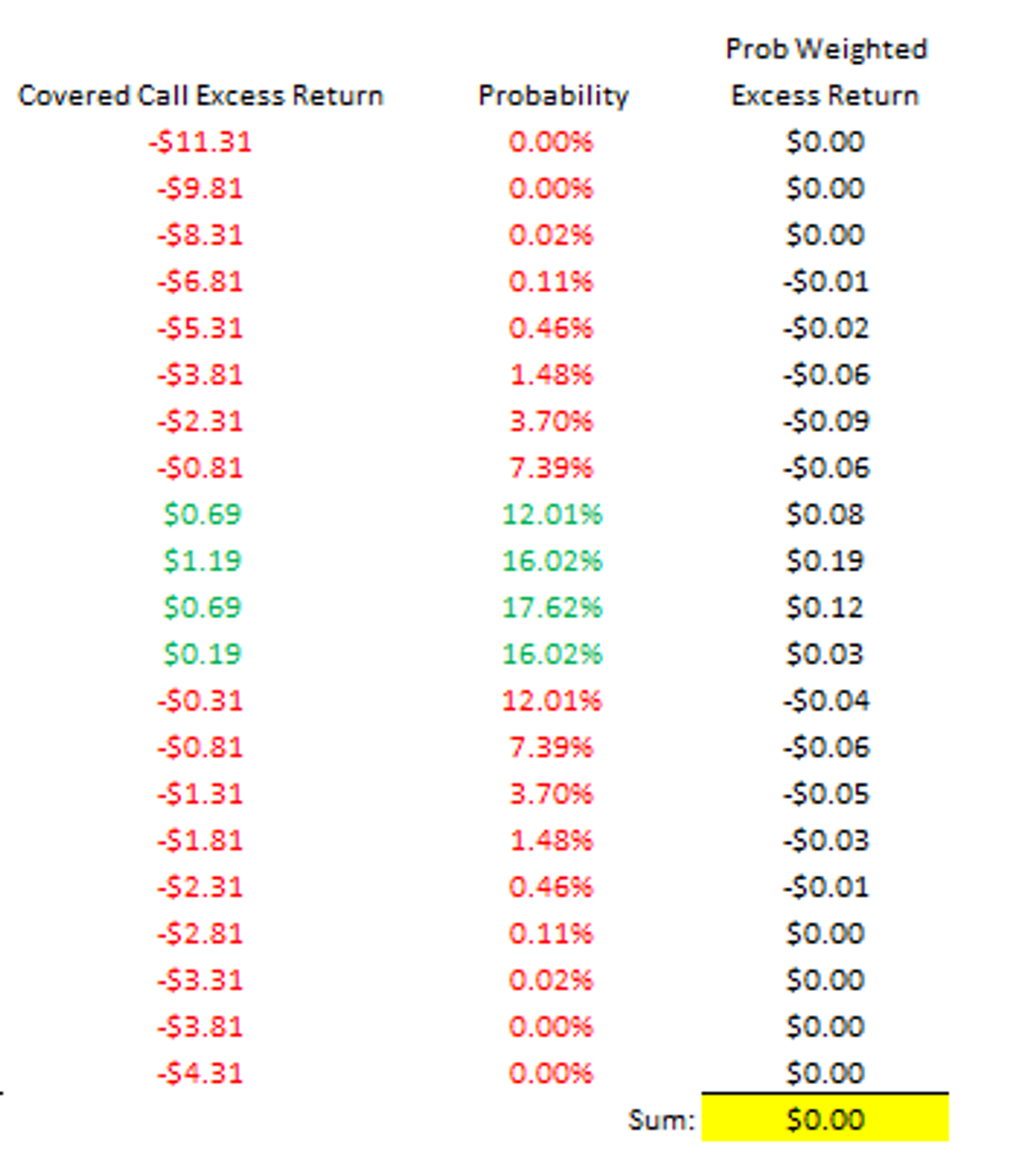
It is handy to create an “excess return” graph that plots the over or underperformance of each portfolio relative to the other at each expiry price. Show the “excess return” chart of the Covered Call portfolio relative to the Reduced Position portfolio.
Answer
This is a handy chart but it’s hiding the fact that even though the covered call strategy has:
has limited outperformance
occurs over only small range of prices
…the strategy outperforms fairly frequently because the range of prices it wins over are the meat of the distribution.
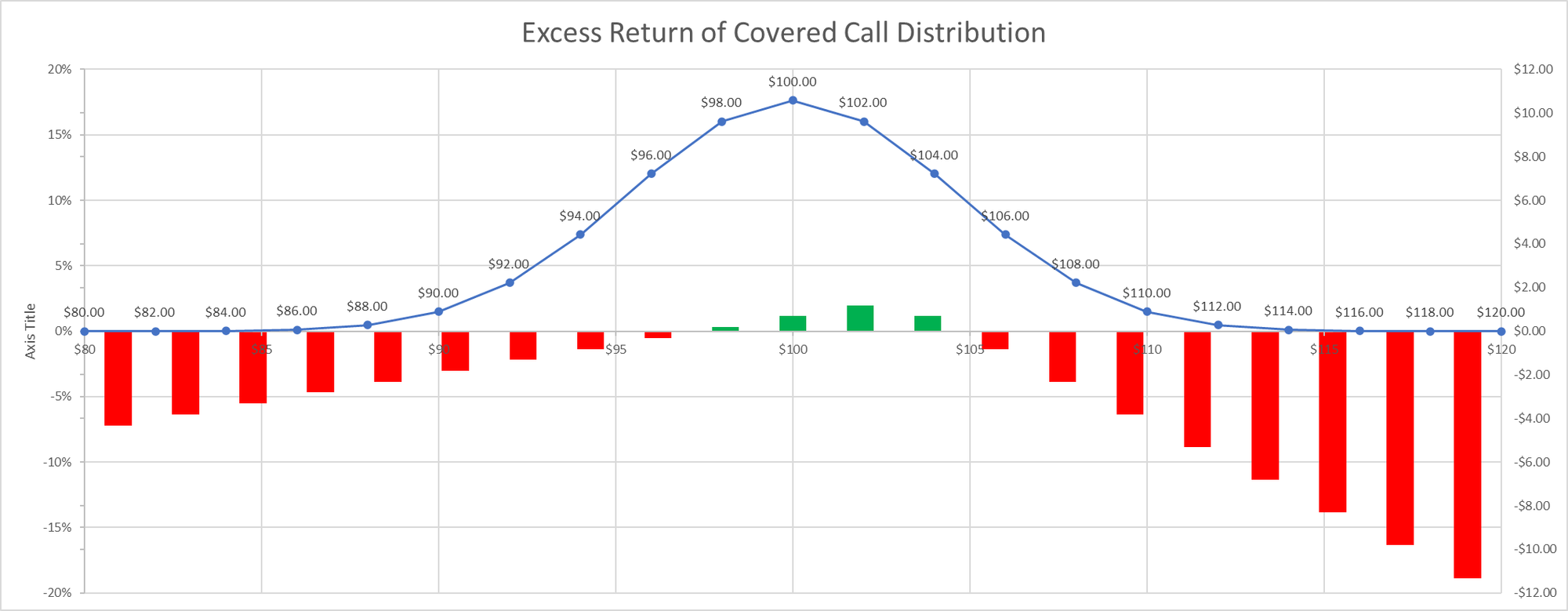
This chart is more revealing:
How often does the Covered Call portfolio outperform the Reduced Position portfolio?
Answer
About 61% Covered Call outperforms Reduced Position
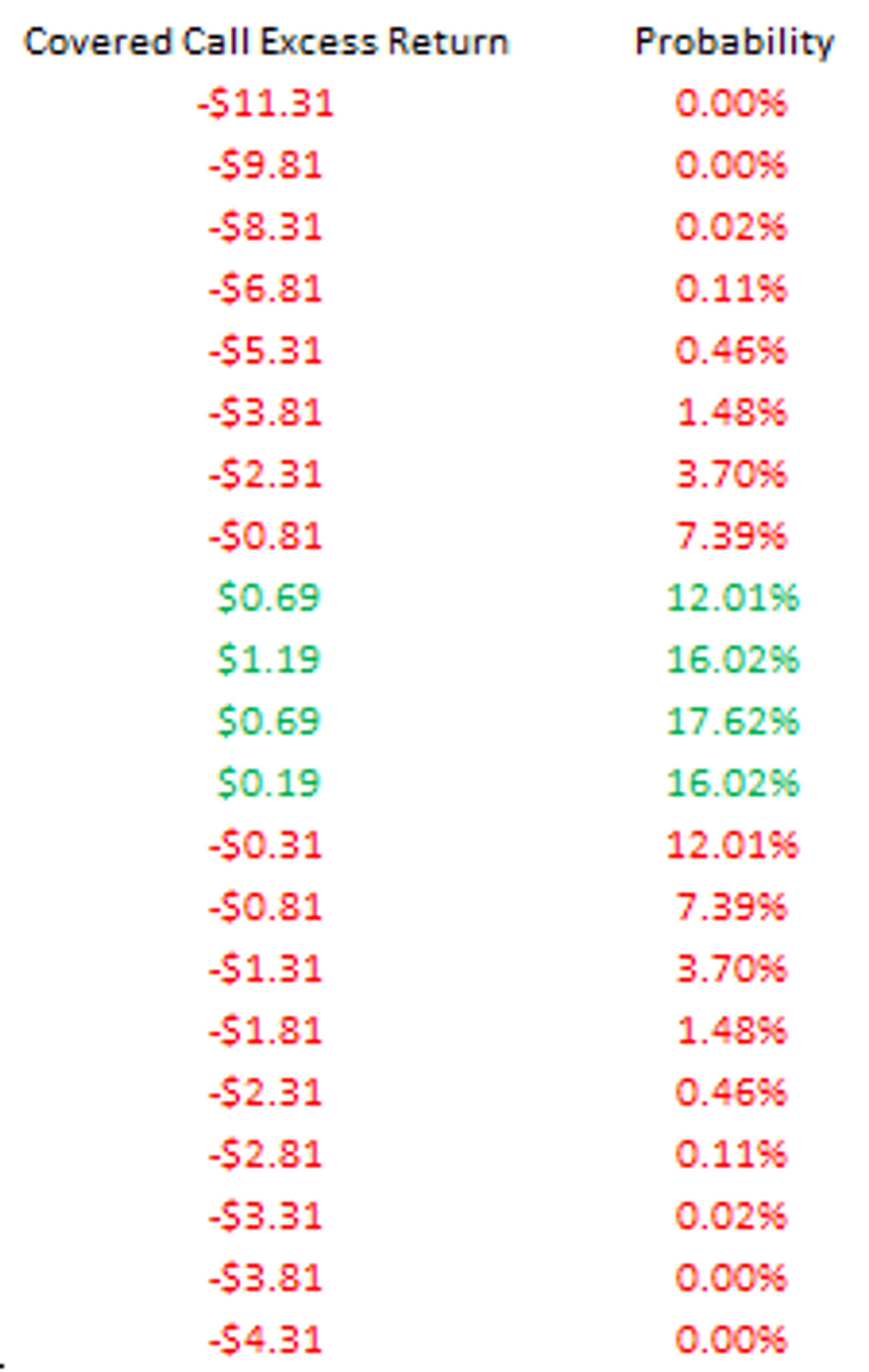
Which portfolio has higher expectancy — Covered Call or Reduced Position?
Answer
It’s a push. This is a tautology — recall that we sold the 103-strike call at a fair value of $.686.
This probability-weighted excess return is 0 confirming our fair value.
🚦
Checkpoint
If we compare selling a covered call to an alternative position where we just sell an equivalent delta worth of shares instead of selling a call, we see a very clear picture.
The covered call strategy is short volatility. It will outperform if the stock doesn’t make a large move and underperform if it does.
It simply doesn’t matter that you sold a call or a put or straddle or a strangle. If you sell an option, you are short volatility even if it’s a covered call or cash secured put.
The outcome of trading an option as opposed to just taking an equivalent option-free exposure will depend on what “volatility” you sold versus what volatility was experienced.
A pedantic caveat
Advanced readers will recognize that it’s a bit more complicated — the path of volatility matters. If you have a covered call position and the underlying experiences extremely high vol but is ultimately unchanged you will still outperform despite being short an option.
Why?
Because you are not dynamically hedging. In other words, you are not “sampling” the higher volatility incurred along the way.
The flip side of this is if you write a covered called and the stock took a trending but low-volatility path, say it went up $.80 a day, then the covered call will do much worse than if you had simply reduced your position size but maintained exposure to the upside. In this case, the volatility was “lower” than what was implied when you sold the 103-call but the trending path made the covered call outcome a disaster.
In sum: you can experience higher or lower realized vol than the implied volatility that you sold based on how frequently you hedge. Every option hedger will “sample” a different realized path.
Over time, the path luck should even out and your p/l approach the spread between the implied you trade in the options and realized vol you hedge at. It’s a noisy process and the less frequently you hedge, the noisier your p/l will be relative to what you will have expected (ie it will take longer to converge.).
The covered call seller doesn’t hedge at all, but as this exercise shows, is still betting on volatility. But there’s so much noise in the process that it’s hard to follow the fuse back to the source of p/l — the relationship of realized volatility to implied volatility. Especially if you make an option trade only 12x per year and don’t hedge.
The book Financial Hacking does an outstanding job of using simple simulations to help you appreciate how noisy the process is and the speed at which it diminishes relative to hedging frequency
In our ongoing example, the option was sold at a fair price assuming the stock would move $1 per day.
The remaining discussion will bootstrap your intuition for how the difference between implied volatility and realized volatility affects even a covered call portfolio held until expiration.
💡
Discussion on how volatility impacts your covered call option trade
We continue to assume you sold the 103-strike call at $.69, the fair value for the option if the stock moves $1 per day. It is rare that you trade an option at exactly the level of volatility the stock realizes until expiration.
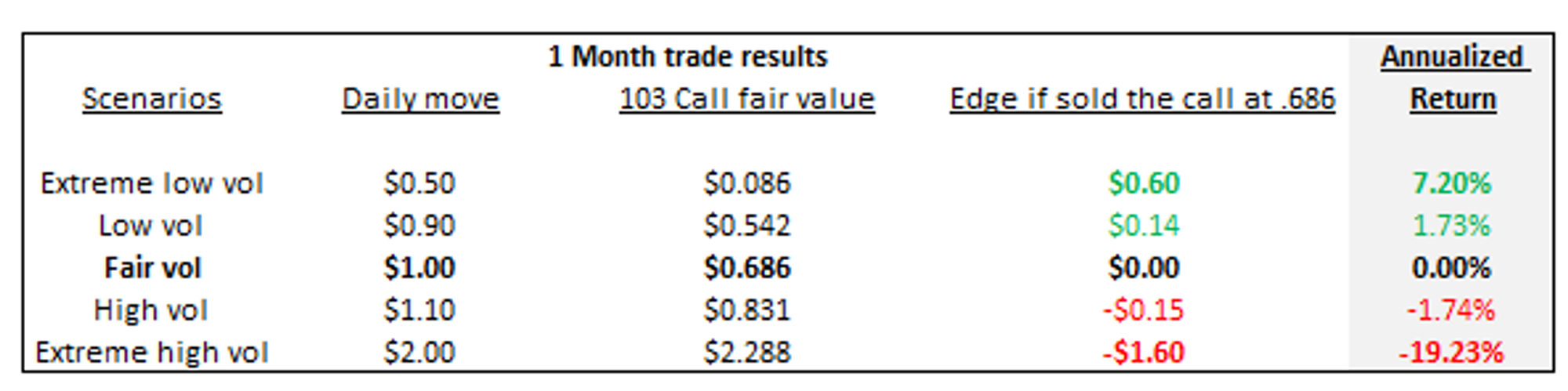
Let’s look at the relative performance of the Covered Call vs Reduced Position for several scenarios. In each scenario we will examine:
Excess return charts showing the p/l of the Covered Call Portfolio minus the Reduced Position, (ie 75% exposure portfolio) at each possible expiration price.
The probability or “hit ratio” of how often the Covered Call Portfolio outperforms the Reduced Position exposure
The expectancy of the Covered Call portfolio based on how much volatility the stock ends up experiencing
Remember, we expected the stock to move $1 per day which gave us a fair value of $.69 for the 103 call. Let’s see what happens when the realized volatility differs.
The skew in the results is what you expect if you decide to sell covered calls instead of just cutting your equity exposure…you are short an option.
The justification for choosing to sell an option should demonstrate why it’s positive expected value to do so. This is not easy. You will experience a high win rate even when you sell the option too cheap (like in the “high vol” scenario). Even in the extremely high-vol scenario where you have made a disastrous trade you still win 1/3 of the time. The gap between win rate and expectancy is where the dragons of marketing and charlatans live.
Options are not cheap to trade. Optically they may appear so but they are highly leveraged — study the table and you can intuit the relationship between those pennies and annualized return. The flip side of this shows why market-making is such a lucrative business. The fraction of a penny you don’t sweat is used to pay for private jets and political influence.
Educationally speaking, put-call parity is not some dry academic idea. It is a profoundly deep insight. It does not matter which specific option expression you choose, the moment you opened an option account you committed to having a view on volatility. All the rhetoric around retail options trading is eliding the fact that the typical option user is poorly equipped to assess if volatility is cheap or expensive and without such a view should not be trading an instrument whose value depends on it.
The pitches all focus on the cadence of your returns…consistent income without confronting what really matters — is the option you are trading the right price? And without a view on volatility, you have no idea.
If you use options to hedge or invest, check out themoontower.ai option trading analytics platform